Укажите функцию с неизвестными коэффициентами, а также данные и найдите коэффициенты в Python
У меня есть функция: f(theta) = a+b*cos(theta - c), а также выборочные данные. Я хотел бы найти коэффициенты a, b и c, которые минимизируют среднеквадратичную ошибку. Любая идея, если есть эффективный способ сделать это в Python?
РЕДАКТИРОВАТЬ:
import numpy as np
from scipy.optimize import curve_fit

#definition of the function
def myfunc(x, a, b, c):
    return a + b * np.cos(x - c)

#sample data
x_data = [0, 60, 120, 180, 240, 300]
y_data = [25, 40, 70, 30, 10, 15]

#the actual curve fitting procedure, a, b, c are stored in popt
popt, _pcov = curve_fit(myfunc, x_data, y_data)
print(popt)
print(np.degrees(popt[2]))

#the rest is just a graphic representation of the data points and the fitted curve
from matplotlib import pyplot as plt

#x_fit = np.linspace(-1, 6, 1000)
y_fit = myfunc(x_data, *popt)

plt.plot(x_data, y_data, "ro")
plt.plot(x_data, y_fit, "b")
plt.xlabel(r'$\theta$ (degrees)');
plt.ylabel(r'$f(\theta)$');

plt.legend()
plt.show()
Вот картинка, показывающая, как кривая не соответствует точкам. Кажется, амплитуда должна быть выше. Местные минимумы и максимумы, кажется, находятся в правильных местах.

1 ответ
scipy.optimize.curve_fit позволяет действительно легко разместить точки данных в вашей пользовательской функции:
import numpy as np
from scipy.optimize import curve_fit

#definition of the function
def myfunc(x, a, b, c):
    return a + b * np.cos(x - c)

#sample data
x_data = np.arange(5)
y_data = 2.34 + 1.23 * np.cos(x_data + .23)

#the actual curve fitting procedure, a, b, c are stored in popt
popt, _pcov = curve_fit(myfunc, x_data, y_data)
print(popt)

#the rest is just a graphic representation of the data points and the fitted curve
from matplotlib import pyplot as plt

x_fit = np.linspace(-1, 6, 1000)
y_fit = myfunc(x_fit, *popt)

plt.plot(x_data, y_data, "ro", label = "data points")
plt.plot(x_fit, y_fit, "b", label = "fitted curve\na = {}\nb = {}\nc = {}".format(*popt))

plt.legend()
plt.show()
Выход:
[ 2.34 1.23 -0.23]
Редактировать:
Обновление вашего вопроса вводит несколько проблем. Во-первых, ваши значения х в градусах, в то время как np.cos ожидает значения в радианах. Поэтому лучше конвертировать значения с np.deg2rad, Обратная функция будет np.rad2deg,
Во-вторых, это хорошая идея для подгонки под разные частоты, давайте введем для этого дополнительный параметр.
В-третьих, приступы обычно довольно чувствительны к первоначальным догадкам. Вы можете предоставить параметр p0 в scipy для этого.
В-четвертых, вы изменили разрешение подобранной кривой на низкое разрешение ваших точек данных, следовательно, оно выглядит слишком слабым. Если мы решим все эти проблемы:
import numpy as np
from scipy.optimize import curve_fit

#sample data
x_data = [0, 60, 120, 180, 240, 300]
y_data = [25, 40, 70, 30, 10, 15]

#definition of the function with additional frequency value d
def myfunc(x, a, b, c, d):
    return a + b * np.cos(d * np.deg2rad(x) - c)
#initial guess of parameters a, b, c, d
p_initial = [np.average(y_data), np.average(y_data), 0, 1]

#the actual curve fitting procedure, a, b, c, d are stored in popt
popt, _pcov = curve_fit(myfunc, x_data, y_data, p0 = p_initial)
print(popt)
#we have to convert the phase shift back into degrees
print(np.rad2deg(popt[2]))

#graphic representation of the data points and the fitted curve
from matplotlib import pyplot as plt
#define x_values for a smooth curve representation
x_fit = np.linspace(np.min(x_data), np.max(x_data), 1000)
y_fit = myfunc(x_fit, *popt)

plt.plot(x_data, y_data, "ro", label = "data")
plt.plot(x_fit, y_fit, "b", label = "fit")
plt.xlabel(r'$\theta$ (degrees)');
plt.ylabel(r'$f(\theta)$');

plt.legend()
plt.show()
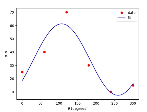
мы получаем этот вывод:
[34.31293761 26.92479369  2.20852009  1.18144319]
126.53888003953764