ggplot2 2.1.0 сломал мой код? Вторичная трансформированная ось теперь отображается неправильно

Question

Некоторое время назад я спросил о добавлении вторичной преобразованной оси x в ggplot, и Нейт Поуп предложил отличное решение, описанное в ggplot2: Добавление вторичной преобразованной оси x поверх графика.

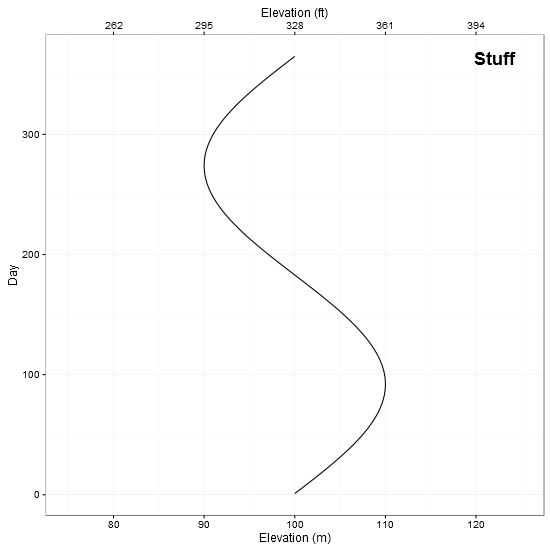
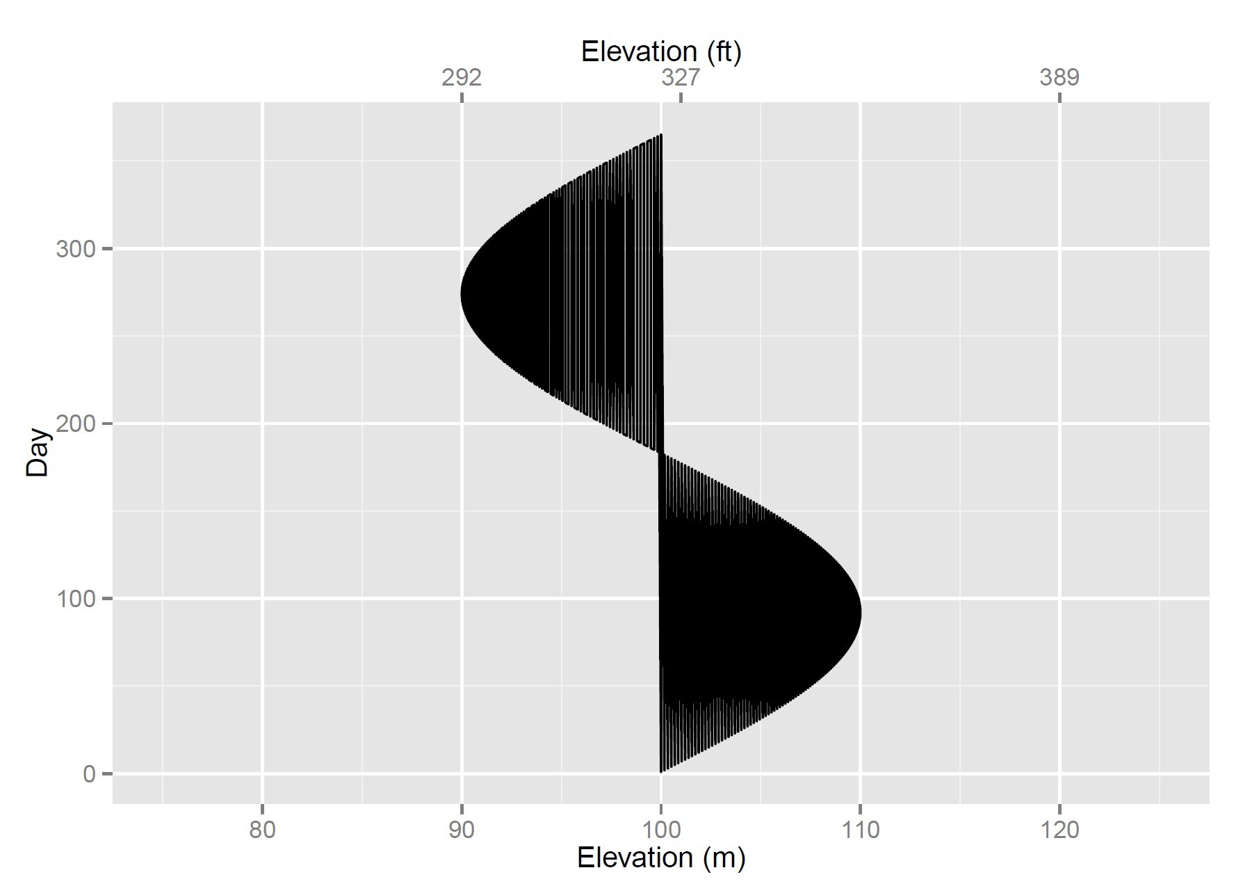
Это решение отлично сработало для меня, и я вернулся к нему, надеясь, что оно подойдет для нового проекта. К сожалению, решение не работает правильно в самой последней версии ggplot2. Теперь выполнение точно такого же кода приводит к "обрезанию" заголовка оси, а также к перекрытию меток и меток. Вот пример с проблемами, выделенными синим цветом:

Этот пример может быть воспроизведен с помощью следующего кода (это точная копия кода Нейта Поупа, который ранее работал изумительно):

library(ggplot2)
library(gtable)
library(grid)

LakeLevels<-data.frame(Day=c(1:365),Elevation=sin(seq(0,2*pi,2*pi/364))*10+100)

## 'base' plot
p1 <- ggplot(data=LakeLevels) + geom_line(aes(x=Elevation,y=Day)) + 
  scale_x_continuous(name="Elevation (m)",limits=c(75,125)) +
  ggtitle("stuff") +
  theme(legend.position="none", plot.title=element_text(hjust=0.94, margin = margin(t = 20, b = -20)))

## plot with "transformed" axis
p2<-ggplot(data=LakeLevels)+geom_line(aes(x=Elevation, y=Day))+
  scale_x_continuous(name="Elevation (ft)", limits=c(75,125),
                     breaks=c(90,101,120),
                     labels=round(c(90,101,120)*3.24084) ## labels convert to feet
  )

## extract gtable
g1 <- ggplot_gtable(ggplot_build(p1))
g2 <- ggplot_gtable(ggplot_build(p2))

## overlap the panel of the 2nd plot on that of the 1st plot
pp <- c(subset(g1$layout, name=="panel", se=t:r))

g <- gtable_add_grob(g1, g2$grobs[[which(g2$layout$name=="panel")]], pp$t, pp$l, pp$b, 
                     pp$l)

g <- gtable_add_grob(g1, g1$grobs[[which(g1$layout$name=="panel")]], pp$t, pp$l, pp$b, pp$l)

## steal axis from second plot and modify
ia <- which(g2$layout$name == "axis-b")
ga <- g2$grobs[[ia]]
ax <- ga$children[[2]]

## switch position of ticks and labels
ax$heights <- rev(ax$heights)
ax$grobs <- rev(ax$grobs)
ax$grobs[[2]]$y <- ax$grobs[[2]]$y - unit(1, "npc") + unit(0.15, "cm")

## modify existing row to be tall enough for axis
g$heights[[2]] <- g$heights[g2$layout[ia,]$t]

## add new axis
g <- gtable_add_grob(g, ax, 2, 4, 2, 4)

## add new row for upper axis label
g <- gtable_add_rows(g, g2$heights[1], 1)
g <- gtable_add_grob(g, g2$grob[[6]], 2, 4, 2, 4)

# draw it
grid.draw(g)

Выполнение приведенного выше кода приводит к двум критическим проблемам, которые я пытаюсь решить:

1) Как отрегулировать ось X, добавленную в верхнюю часть графика, чтобы исправить проблемы с "обрезанием" и перекрытием?

2) Как включить ggtitle("stuff") добавлен в первый сюжет p1 в финальном сюжете?

Я пытался решить эти проблемы весь день, но, похоже, не могу их решить. Буду признателен за любую оказанную помощь. Спасибо!

Answer 1

Обновлен до ggplot2 v 2.2.1, но его проще использовать sec.axis - смотрите здесь

оригинал

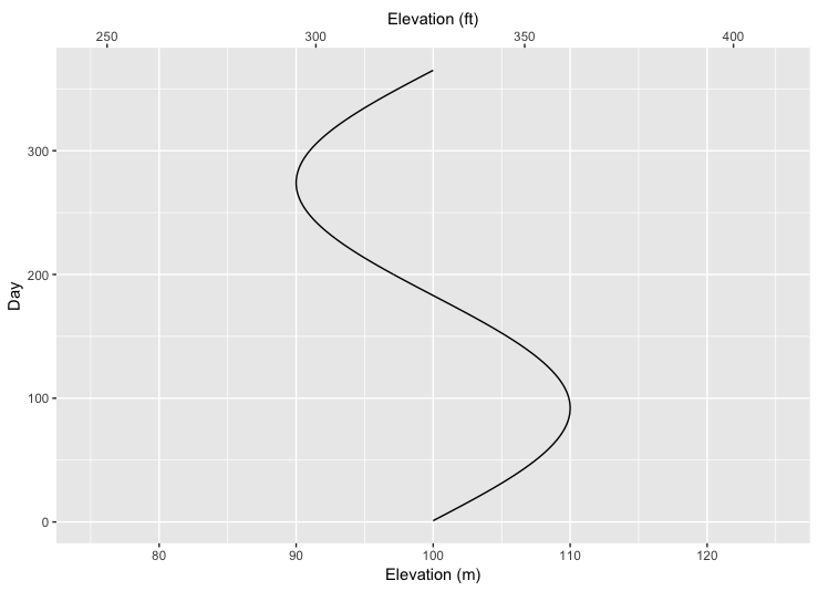
Перемещение осей в ggplot2 стало более сложным с версии 2.1.0. Это решение опирается на код из более старых решений и из кода в cowplot пакет.

Что касается вашего второго вопроса, было легче создать отдельный текстовый гроб для заголовка "Материал" (вместо того, чтобы иметь дело с ggtitle с ее полями).

library(ggplot2) #v 2.2.1
library(gtable)  #v 0.2.0
library(grid)

LakeLevels <- data.frame(Day = c(1:365), Elevation = sin(seq(0, 2*pi, 2 * pi/364)) * 10 + 100)

## 'base' plot
p1 <- ggplot(data = LakeLevels) + 
  geom_path(aes(x = Elevation, y = Day)) + 
  scale_x_continuous(name = "Elevation (m)", limits = c(75, 125)) + 
  theme_bw() 

## plot with "transformed" axis
p2 <- ggplot(data = LakeLevels) +
  geom_path(aes(x = Elevation, y = Day))+
  scale_x_continuous(name = "Elevation (ft)", limits = c(75, 125),
                     breaks = c(80, 90, 100, 110, 120),
                     labels = round(c(80, 90, 100, 110, 120) * 3.28084)) +   ## labels convert to feet
theme_bw()

## Get gtable
g1 <- ggplotGrob(p1)    
g2 <- ggplotGrob(p2)

## Get the position of the plot panel in g1
pp <- c(subset(g1$layout, name == "panel", se = t:r))

# Title grobs have margins. 
# The margins need to be swapped.
# Function to swap margins - 
# taken from the cowplot package:
# https://github.com/wilkelab/cowplot/blob/master/R/switch_axis.R
vinvert_title_grob <- function(grob) {
  heights <- grob$heights
  grob$heights[1] <- heights[3]
  grob$heights[3] <- heights[1]
  grob$vp[[1]]$layout$heights[1] <- heights[3]
  grob$vp[[1]]$layout$heights[3] <- heights[1]

  grob$children[[1]]$hjust <- 1 - grob$children[[1]]$hjust 
  grob$children[[1]]$vjust <- 1 - grob$children[[1]]$vjust 
  grob$children[[1]]$y <- unit(1, "npc") - grob$children[[1]]$y
  grob
}

# Copy "Elevation (ft)" xlab from g2 and swap margins
index <- which(g2$layout$name == "xlab-b")
xlab <- g2$grobs[[index]]
xlab <- vinvert_title_grob(xlab)

# Put xlab at the top of g1
g1 <- gtable_add_rows(g1, g2$heights[g2$layout[index, ]$t], pp$t-1)
g1 <- gtable_add_grob(g1, xlab, pp$t, pp$l, pp$t, pp$r, clip = "off", name="topxlab")

# Get "feet" axis (axis line, tick marks and tick mark labels) from g2
index <- which(g2$layout$name == "axis-b")
xaxis <- g2$grobs[[index]]

# Move the axis line to the bottom (Not needed in your example)
xaxis$children[[1]]$y <- unit.c(unit(0, "npc"), unit(0, "npc"))

# Swap axis ticks and tick mark labels
ticks <- xaxis$children[[2]]
ticks$heights <- rev(ticks$heights)
ticks$grobs <- rev(ticks$grobs)

# Move tick marks
ticks$grobs[[2]]$y <- ticks$grobs[[2]]$y - unit(1, "npc") + unit(3, "pt")

# Sswap tick mark labels' margins
ticks$grobs[[1]] <- vinvert_title_grob(ticks$grobs[[1]])

# Put ticks and tick mark labels back into xaxis
xaxis$children[[2]] <- ticks

# Add axis to top of g1
g1 <- gtable_add_rows(g1, g2$heights[g2$layout[index, ]$t], pp$t)
g1 <- gtable_add_grob(g1, xaxis, pp$t+1, pp$l, pp$t+1, pp$r, clip = "off", name = "axis-t")

# Add "Stuff" title
titleGrob = textGrob("Stuff", x = 0.9, y = 0.95, gp = gpar(cex = 1.5, fontface = "bold"))
g1 <- gtable_add_grob(g1, titleGrob, pp$t+2, pp$l, pp$t+2, pp$r, name = "Title")

# Draw it
grid.newpage()
grid.draw(g1)

Answer 2

Как было предложено выше, вы можете использовать sec_axis или dup_axis.

library(ggplot2)

LakeLevels <- data.frame(Day = c(1:365), 
                         Elevation = sin(seq(0, 2*pi, 2 * pi/364)) * 10 + 100)

ggplot(data = LakeLevels) + 
  geom_path(aes(x = Elevation, y = Day)) + 
  scale_x_continuous(name = "Elevation (m)", limits = c(75, 125),
                     sec.axis = sec_axis(trans = ~ . * 3.28084, name = "Elevation (ft)"))

ggplot2 версия 3.1.1

Answer 3

Подумав немного, я подтвердил, что проблема № 1 возникла из-за изменений в последних версиях ggplot2, и я также нашел временный обходной путь - установка старой версии ggplot2.

После установки более старой версии пакета R для установки ggplot2 1.0.0 я установил ggplot2 1.0.0, используя

packageurl <- "http://cran.r-project.org/src/contrib/Archive/ggplot2/ggplot2_1.0.0.tar.gz"
install.packages(packageurl, repos=NULL, type="source")

с которыми я сверил

packageDescription("ggplot2")$Version

Затем, повторно запустив точный код, указанный выше, я смог создать график с правильно отображенной добавленной осью X:

Это, очевидно, не очень удовлетворительный ответ, но, по крайней мере, он работает, пока кто-то умнее меня не сможет объяснить, почему этот подход не работает в последних версиях ggplot2.:)

Таким образом, проблема № 1 сверху была решена. Я до сих пор не решил проблему № 2 сверху, поэтому буду признателен за понимание этого вопроса.