Как правильно сгладить кривую?

Question

Предположим, у нас есть набор данных, который может быть дан примерно

import numpy as np
x = np.linspace(0,2*np.pi,100)
y = np.sin(x) + np.random.random(100) * 0.2

Поэтому у нас есть вариация 20% набора данных. Моя первая идея заключалась в том, чтобы использовать функцию Scivy UnivariateSpline, но проблема в том, что это не учитывает малый шум в хорошем смысле. Если рассматривать частоты, фон намного меньше сигнала, поэтому сплайном только обрезания может быть идея, но это может включать в себя преобразование Фурье назад и вперед, что может привести к плохому поведению. Другим способом будет скользящее среднее, но для этого также потребуется правильный выбор задержки.

Любые советы / книги или ссылки, как решить эту проблему?

Answer 1

Я предпочитаю фильтр Савицкого-Голея. Он использует метод наименьших квадратов для регрессии небольшого окна ваших данных в полином, а затем использует полином для оценки точки в центре окна. Наконец, окно сдвигается вперед на одну точку данных, и процесс повторяется. Это продолжается до тех пор, пока каждая точка не будет оптимально отрегулирована относительно ее соседей. Он отлично работает даже с шумными выборками из непериодических и нелинейных источников.

Вот подробный пример поваренной книги. Посмотрите мой код ниже, чтобы понять, как легко им пользоваться. Примечание: я пропустил код для определения savitzky_golay() функция, потому что вы можете буквально скопировать / вставить его из примера поваренной книги, который я привел выше.

import numpy as np
import matplotlib.pyplot as plt

x = np.linspace(0,2*np.pi,100)
y = np.sin(x) + np.random.random(100) * 0.2
yhat = savitzky_golay(y, 51, 3) # window size 51, polynomial order 3

plt.plot(x,y)
plt.plot(x,yhat, color='red')
plt.show()

ОБНОВЛЕНИЕ: до меня дошло, что пример поваренной книги, на который я ссылался, был удален. К счастью, фильтр Савицкого-Голея был включен в библиотеку SciPy, на что указывает dodohjk. Чтобы адаптировать приведенный выше код с использованием исходного кода SciPy, введите:

from scipy.signal import savgol_filter
yhat = savgol_filter(y, 51, 3) # window size 51, polynomial order 3

Answer 2

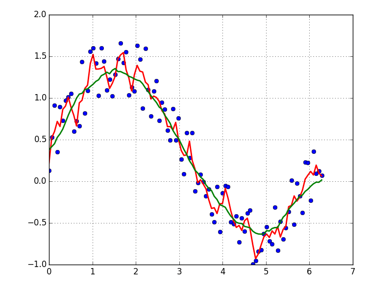
Быстрый и грязный способ сглаживания данных, которые я использую, на основе блока скользящего среднего (по свертке):

x = np.linspace(0,2*np.pi,100)
y = np.sin(x) + np.random.random(100) * 0.8

def smooth(y, box_pts):
    box = np.ones(box_pts)/box_pts
    y_smooth = np.convolve(y, box, mode='same')
    return y_smooth

plot(x, y,'o')
plot(x, smooth(y,3), 'r-', lw=2)
plot(x, smooth(y,19), 'g-', lw=2)

Answer 3

Если вы заинтересованы в "гладкой" версии сигнала, которая является периодической (как ваш пример), тогда БПФ - верный путь. Возьмите преобразование Фурье и вычтите низкочастотные частоты:

import numpy as np
import scipy.fftpack

N = 100
x = np.linspace(0,2*np.pi,N)
y = np.sin(x) + np.random.random(N) * 0.2

w = scipy.fftpack.rfft(y)
f = scipy.fftpack.rfftfreq(N, x[1]-x[0])
spectrum = w**2

cutoff_idx = spectrum < (spectrum.max()/5)
w2 = w.copy()
w2[cutoff_idx] = 0

y2 = scipy.fftpack.irfft(w2)

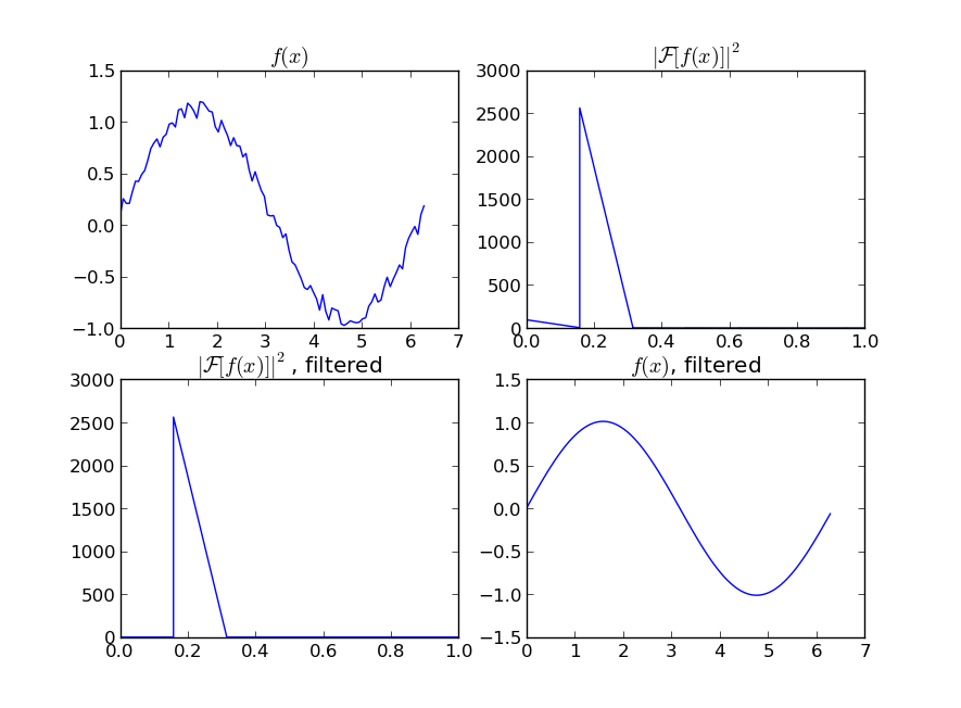
Даже если ваш сигнал не является полностью периодическим, это позволит отлично вычесть белый шум. Существует много типов фильтров (высокочастотный, низкочастотный и т. Д.), Подходящий из которых зависит от того, что вы ищете.

Answer 4

На этот вопрос уже дан подробный ответ, поэтому я думаю, что будет интересен анализ предложенных методов во время выполнения. Я также посмотрю на поведение методов в центре и по краям зашумленного набора данных.

Настроить

Я создал 1000 точек данных в форме кривой греха:

size = 1000
x = np.linspace(0, 4 * np.pi, size)
y = np.sin(x) + np.random.random(size) * 0.2
data = {"time": x, "dummy": y}

Я передаю их в функцию для измерения времени выполнения и построения графика соответствия:

def test_func(f, label):  # f: function handle to one of the smoothing methods
    start = time()
    for i in range(5):
        arr = f(data["dummy"], 20)
    print(f"{label:26s} - time: {time() - start:8.5f} ")
    plt.plot(data["time"], arr, "-", label=label)

Я протестировал множество различных функций сглаживания. arr это массив значений y для сглаживания и spanпараметр сглаживания. Чем ниже, тем лучше соответствие исходным данным, чем выше, тем более гладкой будет полученная кривая.

def smooth_data_convolve_my_average(arr, span):
    re = np.convolve(arr, np.ones(span * 2 + 1) / (span * 2 + 1), mode="same")

    # The "my_average" part: shrinks the averaging window on the side that 
    # reaches beyond the data, keeps the other side the same size as given 
    # by "span"
    re[0] = np.average(arr[:span])
    for i in range(1, span + 1):
        re[i] = np.average(arr[:i + span])
        re[-i] = np.average(arr[-i - span:])
    return re

def smooth_data_np_average(arr, span):  # my original, naive approach
    return [np.average(arr[val - span:val + span + 1]) for val in range(len(arr))]

def smooth_data_np_convolve(arr, span):
    return np.convolve(arr, np.ones(span * 2 + 1) / (span * 2 + 1), mode="same")

def smooth_data_np_cumsum_my_average(arr, span):
    cumsum_vec = np.cumsum(arr)
    moving_average = (cumsum_vec[2 * span:] - cumsum_vec[:-2 * span]) / (2 * span)

    # The "my_average" part again. Slightly different to before, because the
    # moving average from cumsum is shorter than the input and needs to be padded
    front, back = [np.average(arr[:span])], []
    for i in range(1, span):
        front.append(np.average(arr[:i + span]))
        back.insert(0, np.average(arr[-i - span:]))
    back.insert(0, np.average(arr[-2 * span:]))
    return np.concatenate((front, moving_average, back))

def smooth_data_lowess(arr, span):
    x = np.linspace(0, 1, len(arr))
    return sm.nonparametric.lowess(arr, x, frac=(5*span / len(arr)), return_sorted=False)

def smooth_data_kernel_regression(arr, span):
    # "span" smoothing parameter is ignored. If you know how to 
    # incorporate that with kernel regression, please comment below.
    kr = KernelReg(arr, np.linspace(0, 1, len(arr)), 'c')
    return kr.fit()[0]

def smooth_data_savgol_0(arr, span):  
    return savgol_filter(arr, span * 2 + 1, 0)

def smooth_data_savgol_1(arr, span):  
    return savgol_filter(arr, span * 2 + 1, 1)

def smooth_data_savgol_2(arr, span):  
    return savgol_filter(arr, span * 2 + 1, 2)

def smooth_data_fft(arr, span):  # the scaling of "span" is open to suggestions
    w = fftpack.rfft(arr)
    spectrum = w ** 2
    cutoff_idx = spectrum < (spectrum.max() * (1 - np.exp(-span / 2000)))
    w[cutoff_idx] = 0
    return fftpack.irfft(w)

Полученные результаты

Скорость

Runtime over 1000 elements, tested on a python list as well as a numpy array to hold the values.

method              | python list | numpy array
--------------------|-------------|------------
kernel regression   | 23.93405    | 22.75967 
lowess              |  0.61351    |  0.61524 
numpy average       |  0.02485    |  0.02326 
savgol 2            |  0.00186    |  0.00196 
savgol 1            |  0.00157    |  0.00161 
savgol 0            |  0.00155    |  0.00151 
numpy convolve + me |  0.00121    |  0.00115 
numpy cumsum + me   |  0.00114    |  0.00105 
fft                 |  0.00021    |  0.00021 
numpy convolve      |  0.00017    |  0.00015 

Especially kernel regression is very slow to compute over 1k elements, lowess also fails when the dataset becomes much larger. numpy convolve and fft are especially fast. I did not investigate the runtime behavior (O(n)) with increasing or decreasing sample size.

Edge behavior

I'll separate this part into two, to keep image understandable.

Numpy based methods + savgol 0:

These methods calculate an average of the data, the graph is not smoothed. They all (with the exception of numpy.cumsum) result in the same graph when the window that is used to calculate the average does not touch the edge of the data. The discrepancy to numpy.cumsum is most likely due to a 'off by one' error in the window size.

There are different edge behaviours when the method has to work with less data:

• savgol 0: continues with a constant to the edge of the data (savgol 1 and savgol 2 end with a line and parabola respectively)
• numpy average: stops when the window reaches the left side of the data and fills those places in the array with Nan, same behaviour as my_average method on the right side
• numpy convolve: follows the data pretty accurately. I suspect the window size is reduced symmetrically when on side of the window reaches the edge of the data
• my_average/me: my own method that I implemented, because I was not satisfied with the other ones. Simply shrinks the part of the window that is reaching beyond the data to the edge of the data, but keeps the window to the other side the original size given with span

Complicated methods:

These methods all end with a nice fit to the data. savgol 1 ends with a line, savgol 2 with a parabola.

Curve behaviour

To showcase the behaviour of the different methods in the middle of the data.

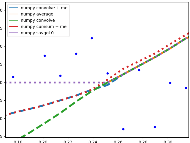
The different savgol and average filters produce a rough line, lowess, fft and kernel regression produce a smooth fit. lowess appears to cut corners when the data changes.

Motivation

I have a Raspberry Pi logging data for fun and the visualization proved to be a small challenge. All data points, except RAM usage and ethernet traffic are only recorded in discrete steps and/or inherently noisy. For example the temperature sensor only outputs whole degrees, but differs by up to two degrees between consecutive measurements. No useful information can be gained from such a scatter plot. To visualize the data I therefore needed some method that is not too computationally expensive and produced a moving average. I also wanted nice behavior at the edges of the data, as this especially impacts the latest info when looking at live data. I settled on the numpy convolve method with my_average to improve the edge behavior.

Answer 5

Подгонка скользящего среднего к вашим данным сгладит шум, посмотрите этот ответ, чтобы узнать, как это сделать.

Если вы хотите использовать LOWESS, чтобы соответствовать вашим данным (это похоже на скользящее среднее, но более изощренно), вы можете сделать это с помощью библиотеки statsmodels:

import numpy as np
import pylab as plt
import statsmodels.api as sm

x = np.linspace(0,2*np.pi,100)
y = np.sin(x) + np.random.random(100) * 0.2
lowess = sm.nonparametric.lowess(y, x, frac=0.1)

plt.plot(x, y, '+')
plt.plot(lowess[:, 0], lowess[:, 1])
plt.show()

Наконец, если вы знаете функциональную форму вашего сигнала, вы можете подогнать кривую к вашим данным, что, вероятно, будет лучшим решением.

Answer 6

Другой вариант - использовать KernelReg в statsmodel:

from statsmodels.nonparametric.kernel_regression import KernelReg
import numpy as np
import matplotlib.pyplot as plt
x = np.linspace(0,2*np.pi,100)
y = np.sin(x) + np.random.random(100) * 0.2
# The third parameter specifies the type of the variable x;
# 'c' stands for continuous
kr = KernelReg(y,x,'c')
plt.plot(x, y, '+')
y_pred, y_std = kr.fit(x)
plt.plot(x, y_pred)
plt.show()

Answer 7

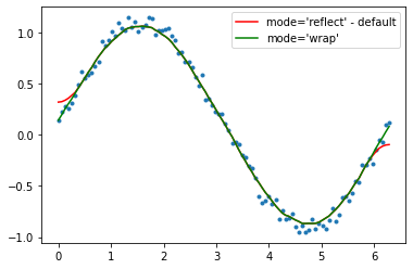
Проверь это! Существует четкое определение сглаживания 1D сигнала.

http://scipy-cookbook.readthedocs.io/items/SignalSmooth.html

Клавиши быстрого доступа:

import numpy

def smooth(x,window_len=11,window='hanning'):
    """smooth the data using a window with requested size.

    This method is based on the convolution of a scaled window with the signal.
    The signal is prepared by introducing reflected copies of the signal 
    (with the window size) in both ends so that transient parts are minimized
    in the begining and end part of the output signal.

    input:
        x: the input signal 
        window_len: the dimension of the smoothing window; should be an odd integer
        window: the type of window from 'flat', 'hanning', 'hamming', 'bartlett', 'blackman'
            flat window will produce a moving average smoothing.

    output:
        the smoothed signal

    example:

    t=linspace(-2,2,0.1)
    x=sin(t)+randn(len(t))*0.1
    y=smooth(x)

    see also: 

    numpy.hanning, numpy.hamming, numpy.bartlett, numpy.blackman, numpy.convolve
    scipy.signal.lfilter

    TODO: the window parameter could be the window itself if an array instead of a string
    NOTE: length(output) != length(input), to correct this: return y[(window_len/2-1):-(window_len/2)] instead of just y.
    """

    if x.ndim != 1:
        raise ValueError, "smooth only accepts 1 dimension arrays."

    if x.size < window_len:
        raise ValueError, "Input vector needs to be bigger than window size."


    if window_len<3:
        return x


    if not window in ['flat', 'hanning', 'hamming', 'bartlett', 'blackman']:
        raise ValueError, "Window is on of 'flat', 'hanning', 'hamming', 'bartlett', 'blackman'"


    s=numpy.r_[x[window_len-1:0:-1],x,x[-2:-window_len-1:-1]]
    #print(len(s))
    if window == 'flat': #moving average
        w=numpy.ones(window_len,'d')
    else:
        w=eval('numpy.'+window+'(window_len)')

    y=numpy.convolve(w/w.sum(),s,mode='valid')
    return y




from numpy import *
from pylab import *

def smooth_demo():

    t=linspace(-4,4,100)
    x=sin(t)
    xn=x+randn(len(t))*0.1
    y=smooth(x)

    ws=31

    subplot(211)
    plot(ones(ws))

    windows=['flat', 'hanning', 'hamming', 'bartlett', 'blackman']

    hold(True)
    for w in windows[1:]:
        eval('plot('+w+'(ws) )')

    axis([0,30,0,1.1])

    legend(windows)
    title("The smoothing windows")
    subplot(212)
    plot(x)
    plot(xn)
    for w in windows:
        plot(smooth(xn,10,w))
    l=['original signal', 'signal with noise']
    l.extend(windows)

    legend(l)
    title("Smoothing a noisy signal")
    show()


if __name__=='__main__':
    smooth_demo()

Answer 8

Для моего проекта мне нужно было создать интервалы для моделирования временных рядов, и чтобы сделать процедуру более эффективной, я создал tsmoothie: библиотеку Python для сглаживания временных рядов и обнаружения выбросов векторизованным способом.

Он предоставляет различные алгоритмы сглаживания вместе с возможностью вычисления интервалов.

Здесь я использую ConvolutionSmoother но вы также можете проверить это на других.

      import numpy as np
import matplotlib.pyplot as plt
from tsmoothie.smoother import *

x = np.linspace(0,2*np.pi,100)
y = np.sin(x) + np.random.random(100) * 0.2

# operate smoothing
smoother = ConvolutionSmoother(window_len=5, window_type='ones')
smoother.smooth(y)

# generate intervals
low, up = smoother.get_intervals('sigma_interval', n_sigma=2)

# plot the smoothed timeseries with intervals
plt.figure(figsize=(11,6))
plt.plot(smoother.smooth_data[0], linewidth=3, color='blue')
plt.plot(smoother.data[0], '.k')
plt.fill_between(range(len(smoother.data[0])), low[0], up[0], alpha=0.3)

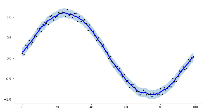
Я также отмечаю, что tsmoothie может выполнять сглаживание нескольких таймсерий векторизованным способом.

Answer 9

Есть простая функцияscipy.ndimageэто также хорошо работает для меня:

      from scipy.ndimage import uniform_filter1d

y_smooth = uniform_filter1d(y,size=15)

Answer 10

Вы также можете использовать это:

      def smooth(scalars, weight = 0.8):  # Weight between 0 and 1
        return [scalars[i] * weight + (1 - weight) * scalars[i+1] for i in range(len(scalars)) if i < len(scalars)-1]

Answer 11

Быстрый способ использования скользящей средней (который также работает для небиективных функций):

      def smoothen(x, winsize=5):
    return np.array(pd.Series(x).rolling(winsize).mean())[winsize-1:]

Этот код основан на https://towardsdatascience.com/data-smoothing-for-data-science-visualization-the-goldilocks-trio-part-1-867765050615. Там же обсуждаются более продвинутые решения.

Answer 12

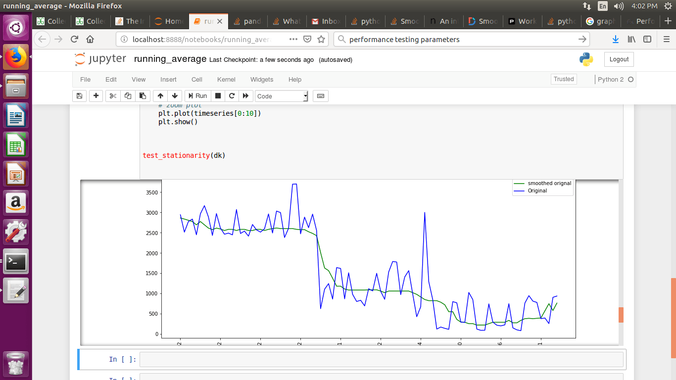
Если вы строите график временных рядов и используете mtplotlib для рисования графиков, используйте метод медианы для сглаживания графика.

smotDeriv = timeseries.rolling(window=20, min_periods=5, center=True).median()

где timeseries ваш набор данных передан, вы можете изменить windowsize для более сглаживания.