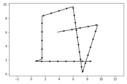
Как мне указать стреловидный стиль линии в Matplotlib?
Я хотел бы отобразить набор данных xy в Matplotlib таким образом, чтобы указать конкретный путь. В идеале, стиль линии должен быть изменен, чтобы использовать патч, похожий на стрелку. Я создал макет, показанный ниже (используя Omnigraphsketcher). Кажется, я должен иметь возможность переопределить один из общих linestyle декларации ('-', '--', ':'и т. д.) на этот счет.
Обратите внимание, что я НЕ хочу просто соединять каждую точку данных одной стрелкой - на самом деле точки данных не распределены равномерно, и мне нужно постоянное расстояние между стрелками.

5 ответов
Вот отправная точка:
Идите вдоль своей линии на фиксированных шагах (
aspaceв моем примере ниже) .О. Это включает в себя выполнение шагов вдоль отрезков, созданных двумя наборами точек (
x1,y1) а также (x2,y2) .B. Если ваш шаг длиннее отрезка, переходите к следующему набору точек.
В этот момент определите угол наклона линии.
Нарисуйте стрелку с наклоном, соответствующим углу.
Я написал небольшой сценарий, чтобы продемонстрировать это:
import numpy as np
import matplotlib.pyplot as plt

fig = plt.figure()
axes = fig.add_subplot(111)

# my random data
scale = 10
np.random.seed(101)
x = np.random.random(10)*scale
y = np.random.random(10)*scale

# spacing of arrows
aspace = .1 # good value for scale of 1
aspace *= scale

# r is the distance spanned between pairs of points
r = [0]
for i in range(1,len(x)):
    dx = x[i]-x[i-1]
    dy = y[i]-y[i-1]
    r.append(np.sqrt(dx*dx+dy*dy))
r = np.array(r)

# rtot is a cumulative sum of r, it's used to save time
rtot = []
for i in range(len(r)):
    rtot.append(r[0:i].sum())
rtot.append(r.sum())

arrowData = [] # will hold tuples of x,y,theta for each arrow
arrowPos = 0 # current point on walk along data
rcount = 1
while arrowPos < r.sum():
    x1,x2 = x[rcount-1],x[rcount]
    y1,y2 = y[rcount-1],y[rcount]
    da = arrowPos-rtot[rcount]
    theta = np.arctan2((x2-x1),(y2-y1))
    ax = np.sin(theta)*da+x1
    ay = np.cos(theta)*da+y1
    arrowData.append((ax,ay,theta))
    arrowPos+=aspace
    while arrowPos > rtot[rcount+1]:
        rcount+=1
        if arrowPos > rtot[-1]:
            break

# could be done in above block if you want
for ax,ay,theta in arrowData:
    # use aspace as a guide for size and length of things
    # scaling factors were chosen by experimenting a bit
    axes.arrow(ax,ay,
               np.sin(theta)*aspace/10,np.cos(theta)*aspace/10,
               head_width=aspace/8)


axes.plot(x,y)
axes.set_xlim(x.min()*.9,x.max()*1.1)
axes.set_ylim(y.min()*.9,y.max()*1.1)

plt.show()
Этот пример приводит к следующему рисунку: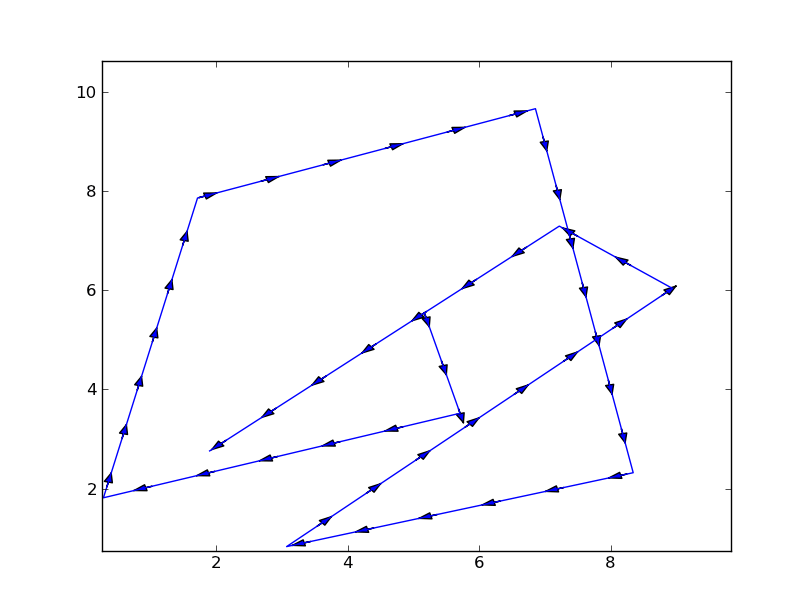
Здесь есть много возможностей для совершенствования:
- Можно использовать FancyArrowPatch для настройки внешнего вида стрелок.
- При создании стрелок можно добавить дополнительный тест, чтобы убедиться, что они не выходят за пределы линии. Это будет иметь отношение к стрелкам, созданным в или около вершины, где линия резко меняет направление. Это относится к самой правой точке выше.
- Из этого скрипта можно создать метод, который будет работать в более широком диапазоне случаев, т.е. сделать его более переносимым.
Посмотрев на это, я обнаружил способ построения колчана. Это могло бы быть в состоянии заменить вышеупомянутую работу, но не было сразу очевидно, что это было гарантировано.
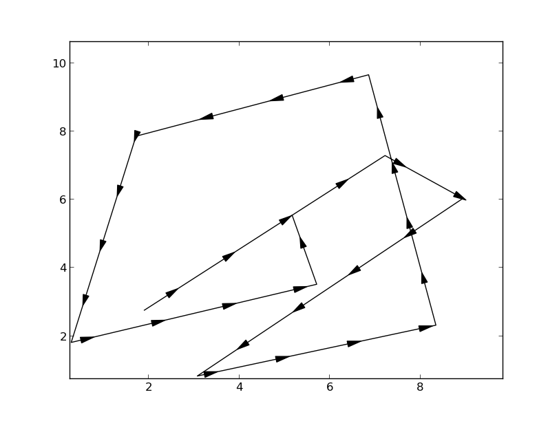
Очень хороший ответ от Yann, но с помощью стрелки на получающиеся стрелки могут влиять соотношение сторон и пределы осей. Я сделал версию, которая использует axes.annotate() вместо axes.arrow(). Я включил это здесь для других, чтобы использовать.
Вкратце это используется для построения стрелок вдоль ваших линий в matplotlib. Код показан ниже. Это все еще можно улучшить, добавив возможность иметь разные стрелки. Здесь я только включил контроль ширины и длины стрелки.
import numpy as np
import matplotlib.pyplot as plt


def arrowplot(axes, x, y, narrs=30, dspace=0.5, direc='pos', \
                          hl=0.3, hw=6, c='black'):
    ''' narrs  :  Number of arrows that will be drawn along the curve

        dspace :  Shift the position of the arrows along the curve.
                  Should be between 0. and 1.

        direc  :  can be 'pos' or 'neg' to select direction of the arrows

        hl     :  length of the arrow head

        hw     :  width of the arrow head

        c      :  color of the edge and face of the arrow head
    '''

    # r is the distance spanned between pairs of points
    r = [0]
    for i in range(1,len(x)):
        dx = x[i]-x[i-1]
        dy = y[i]-y[i-1]
        r.append(np.sqrt(dx*dx+dy*dy))
    r = np.array(r)

    # rtot is a cumulative sum of r, it's used to save time
    rtot = []
    for i in range(len(r)):
        rtot.append(r[0:i].sum())
    rtot.append(r.sum())

    # based on narrs set the arrow spacing
    aspace = r.sum() / narrs

    if direc is 'neg':
        dspace = -1.*abs(dspace)
    else:
        dspace = abs(dspace)

    arrowData = [] # will hold tuples of x,y,theta for each arrow
    arrowPos = aspace*(dspace) # current point on walk along data
                                 # could set arrowPos to 0 if you want
                                 # an arrow at the beginning of the curve

    ndrawn = 0
    rcount = 1
    while arrowPos < r.sum() and ndrawn < narrs:
        x1,x2 = x[rcount-1],x[rcount]
        y1,y2 = y[rcount-1],y[rcount]
        da = arrowPos-rtot[rcount]
        theta = np.arctan2((x2-x1),(y2-y1))
        ax = np.sin(theta)*da+x1
        ay = np.cos(theta)*da+y1
        arrowData.append((ax,ay,theta))
        ndrawn += 1
        arrowPos+=aspace
        while arrowPos > rtot[rcount+1]:
            rcount+=1
            if arrowPos > rtot[-1]:
                break

    # could be done in above block if you want
    for ax,ay,theta in arrowData:
        # use aspace as a guide for size and length of things
        # scaling factors were chosen by experimenting a bit

        dx0 = np.sin(theta)*hl/2. + ax
        dy0 = np.cos(theta)*hl/2. + ay
        dx1 = -1.*np.sin(theta)*hl/2. + ax
        dy1 = -1.*np.cos(theta)*hl/2. + ay

        if direc is 'neg' :
          ax0 = dx0
          ay0 = dy0
          ax1 = dx1
          ay1 = dy1
        else:
          ax0 = dx1
          ay0 = dy1
          ax1 = dx0
          ay1 = dy0

        axes.annotate('', xy=(ax0, ay0), xycoords='data',
                xytext=(ax1, ay1), textcoords='data',
                arrowprops=dict( headwidth=hw, frac=1., ec=c, fc=c))


    axes.plot(x,y, color = c)
    axes.set_xlim(x.min()*.9,x.max()*1.1)
    axes.set_ylim(y.min()*.9,y.max()*1.1)


if __name__ == '__main__':
    fig = plt.figure()
    axes = fig.add_subplot(111)

    # my random data
    scale = 10
    np.random.seed(101)
    x = np.random.random(10)*scale
    y = np.random.random(10)*scale
    arrowplot(axes, x, y )

    plt.show()
Полученную цифру можно увидеть здесь:
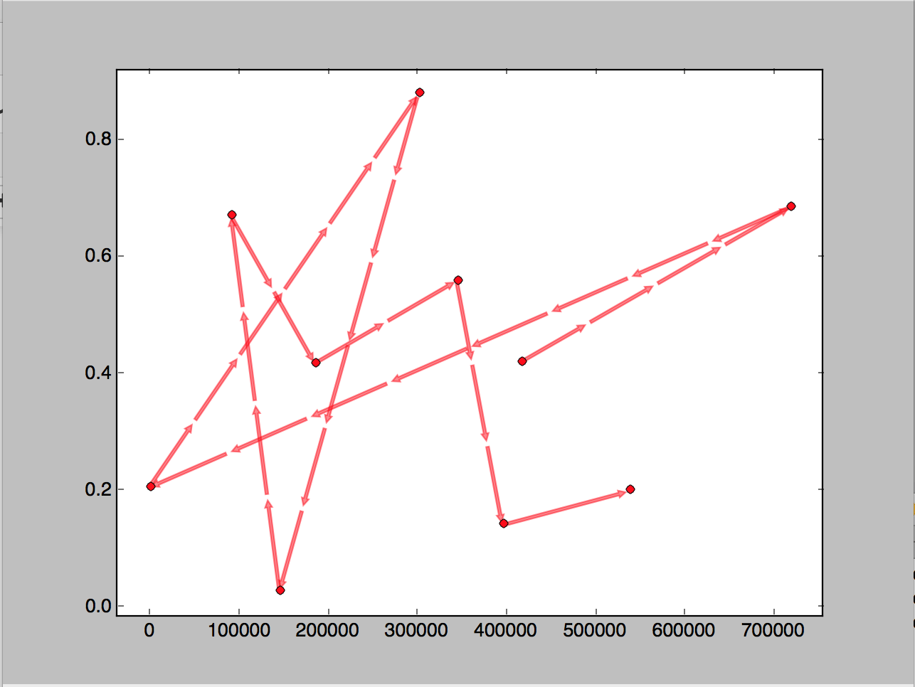
Вот модифицированная и оптимизированная версия кода Дуарте. У меня были проблемы, когда я запускал его код с различными наборами данных и форматами изображения, поэтому я очистил его и использовал FancyArrowPatches для стрелок. Обратите внимание, что пример графика имеет масштаб в 1000000 раз отличающийся по x от y.
Я также переключился на рисование стрелки в отображаемых координатах, чтобы различное масштабирование по осям x и y не изменило длины стрелки.
Попутно я обнаружил ошибку в FancyArrowPatch в matplotlib, которая бомбит при построении чисто вертикальной стрелки. Я нашел обходной путь, который есть в моем коде.
import numpy as np
import matplotlib.pyplot as plt
import matplotlib.patches as patches


def arrowplot(axes, x, y, nArrs=30, mutateSize=10, color='gray', markerStyle='o'):
    '''arrowplot : plots arrows along a path on a set of axes
        axes   :  the axes the path will be plotted on
        x      :  list of x coordinates of points defining path
        y      :  list of y coordinates of points defining path
        nArrs  :  Number of arrows that will be drawn along the path
        mutateSize :  Size parameter for arrows
        color  :  color of the edge and face of the arrow head
        markerStyle : Symbol

        Bugs: If a path is straight vertical, the matplotlab FanceArrowPatch bombs out.
          My kludge is to test for a vertical path, and perturb the second x value
          by 0.1 pixel. The original x & y arrays are not changed

        MHuster 2016, based on code by
    '''
    # recast the data into numpy arrays
    x = np.array(x, dtype='f')
    y = np.array(y, dtype='f')
    nPts = len(x)

    # Plot the points first to set up the display coordinates
    axes.plot(x,y, markerStyle, ms=5, color=color)

    # get inverse coord transform
    inv = ax.transData.inverted()

    # transform x & y into display coordinates
    # Variable with a 'D' at the end are in display coordinates
    xyDisp = np.array(axes.transData.transform(zip(x,y)))
    xD = xyDisp[:,0]
    yD = xyDisp[:,1]

    # drD is the distance spanned between pairs of points
    # in display coordinates
    dxD = xD[1:] - xD[:-1]
    dyD = yD[1:] - yD[:-1]
    drD = np.sqrt(dxD**2 + dyD**2)

    # Compensating for matplotlib bug
    dxD[np.where(dxD==0.0)] = 0.1


    # rtotS is the total path length
    rtotD = np.sum(drD)

    # based on nArrs, set the nominal arrow spacing
    arrSpaceD = rtotD / nArrs

    # Loop over the path segments
    iSeg = 0
    while iSeg < nPts - 1:
        # Figure out how many arrows in this segment.
        # Plot at least one.
        nArrSeg = max(1, int(drD[iSeg] / arrSpaceD + 0.5))
        xArr = (dxD[iSeg]) / nArrSeg # x size of each arrow
        segSlope = dyD[iSeg] / dxD[iSeg]
        # Get display coordinates of first arrow in segment
        xBeg = xD[iSeg]
        xEnd = xBeg + xArr
        yBeg = yD[iSeg]
        yEnd = yBeg + segSlope * xArr
        # Now loop over the arrows in this segment
        for iArr in range(nArrSeg):
            # Transform the oints back to data coordinates
            xyData = inv.transform(((xBeg, yBeg),(xEnd,yEnd)))
            # Use a patch to draw the arrow
            # I draw the arrows with an alpha of 0.5
            p = patches.FancyArrowPatch(
                xyData[0], xyData[1],
                arrowstyle='simple',
                mutation_scale=mutateSize,
                color=color, alpha=0.5)
            axes.add_patch(p)
            # Increment to the next arrow
            xBeg = xEnd
            xEnd += xArr
            yBeg = yEnd
            yEnd += segSlope * xArr
        # Increment segment number
        iSeg += 1

if __name__ == '__main__':
    import numpy as np
    import matplotlib.pyplot as plt
    fig = plt.figure()
    ax = fig.add_subplot(111)
    # my random data
    xScale = 1e6
    np.random.seed(1)
    x = np.random.random(10) * xScale
    y = np.random.random(10)
    arrowplot(ax, x, y, nArrs=4*(len(x)-1), mutateSize=10, color='red')
    xRng = max(x) - min(x)
    ax.set_xlim(min(x) - 0.05*xRng, max(x) + 0.05*xRng)
    yRng = max(y) - min(y)
    ax.set_ylim(min(y) - 0.05*yRng, max(y) + 0.05*yRng)
    plt.show()
Векторизованная версия ответа Янна:
import numpy as np
import matplotlib.pyplot as plt

def distance(data):
    return np.sum((data[1:] - data[:-1]) ** 2, axis=1) ** .5

def draw_path(path):
    HEAD_WIDTH = 2
    HEAD_LEN = 3

    fig = plt.figure()
    axes = fig.add_subplot(111)

    x = path[:,0]
    y = path[:,1]
    axes.plot(x, y)

    theta = np.arctan2(y[1:] - y[:-1], x[1:] - x[:-1])
    dist = distance(path) - HEAD_LEN

    x = x[:-1]
    y = y[:-1]
    ax = x + dist * np.sin(theta)
    ay = y + dist * np.cos(theta)

    for x1, y1, x2, y2 in zip(x,y,ax-x,ay-y):
        axes.arrow(x1, y1, x2, y2, head_width=HEAD_WIDTH, head_length=HEAD_LEN)
    plt.show()
Если вы можете жить без причудливых стрелок, огибающих край / фиксированной длины, вот версия для бедняков, погружающая сегменты прибл. длинные отрезки. Если
ds не слишком велика, на мой взгляд, разница незначительна.
      from matplotlib import pyplot as plt
import numpy as np

np.random.seed(42)
x, y = 10*np.random.rand(2,8)

# length of line segment
ds=1

# number of line segments per interval
Ns = np.round(np.sqrt( (x[1:]-x[:-1])**2 + (y[1:]-y[:-1])**2 ) / ds).astype(int)

# sub-divide intervals w.r.t. Ns
subdiv = lambda x, Ns=Ns: np.concatenate([ np.linspace(x[ii], x[ii+1], Ns[ii]) for ii, _ in enumerate(x[:-1]) ])

x, y = subdiv(x), subdiv(y)

plt.quiver(x[:-1], y[:-1], x[1:]-x[:-1], y[1:]-y[:-1], scale_units='xy', angles='xy', scale=1, width=.004, headlength=4, headwidth=4)