Построить регрессионный биплот частичных наименьших квадратов с помощью ggplot2
С использованием data.frame ниже (Источник: http://eric.univ-lyon2.fr/~ricco/tanagra/fichiers/en_Tanagra_PLSR_Software_Comparison.pdf)
Данные
df <- read.table(text = c("
diesel  twodoors    sportsstyle wheelbase   length  width   height  curbweight  enginesize  horsepower  horse_per_weight    conscity    price   symboling
0   1   0   97  172 66  56  2209    109 85  0.0385  8.7 7975    2
0   0   0   100 177 66  54  2337    109 102 0.0436  9.8 13950   2
0   0   0   116 203 72  57  3740    234 155 0.0414  14.7    34184   -1
0   1   1   103 184 68  52  3016    171 161 0.0534  12.4    15998   3
0   0   0   101 177 65  54  2765    164 121 0.0438  11.2    21105   0
0   1   0   90  169 65  52  2756    194 207 0.0751  13.8    34028   3
1   0   0   105 175 66  54  2700    134 72  0.0267  7.6 18344   0
0   0   0   108 187 68  57  3020    120 97  0.0321  12.4    11900   0
0   0   1   94  157 64  51  1967    90  68  0.0346  7.6 6229    1
0   1   0   95  169 64  53  2265    98  112 0.0494  9.0 9298    1
1   0   0   96  166 64  53  2275    110 56  0.0246  6.9 7898    0
0   1   0   100 177 66  53  2507    136 110 0.0439  12.4    15250   2
0   1   1   94  157 64  51  1876    90  68  0.0362  6.4 5572    1
0   0   0   95  170 64  54  2024    97  69  0.0341  7.6 7349    1
0   1   1   95  171 66  52  2823    152 154 0.0546  12.4    16500   1
0   0   0   103 175 65  60  2535    122 88  0.0347  9.8 8921    -1
0   0   0   113 200 70  53  4066    258 176 0.0433  15.7    32250   0
0   0   0   95  165 64  55  1938    97  69  0.0356  7.6 6849    1
1   0   0   97  172 66  56  2319    97  68  0.0293  6.4 9495    2
0   0   0   97  172 66  56  2275    109 85  0.0374  8.7 8495    2"), header = T)
и это
Код
library(plsdepot)
df.plsdepot = plsreg1(df[, 1:11], df[, 14, drop = FALSE], comps = 3)
plot(df.plsdepot, comps = c(1, 2))
Я получил это
Результат
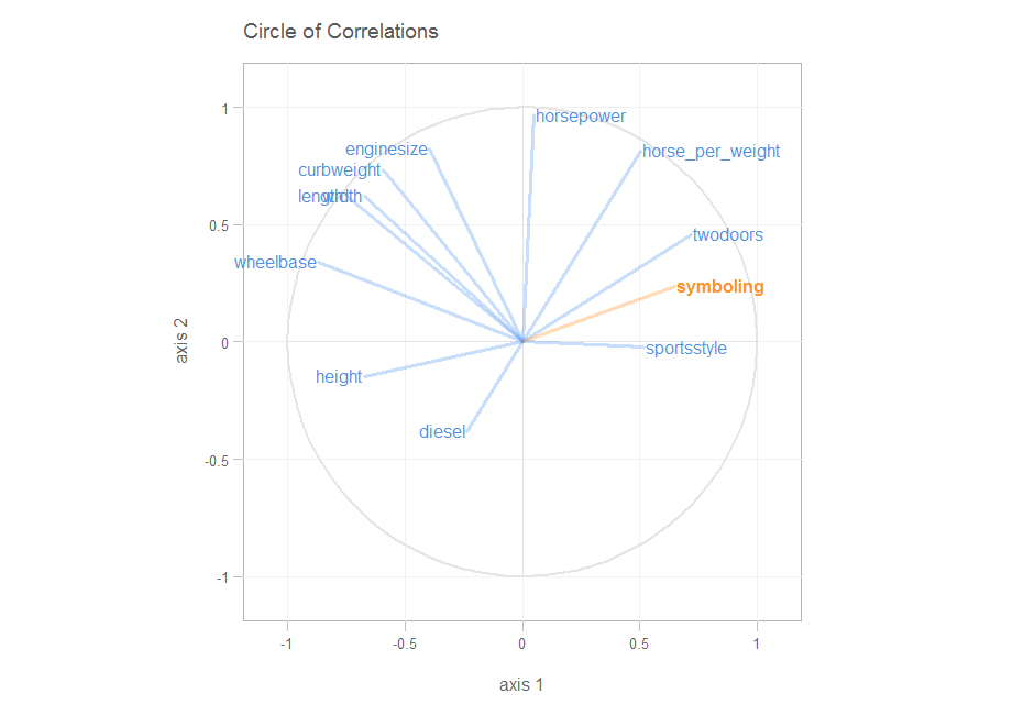
Зависимая (y) переменная здесь symboling, как и цена, является функцией всех других независимых переменных для автомобилей (diesel, twodoors, sportsstyle, wheelbase, length, width, height, curbweight, enginesize,horsepower, horse_per_weight)
Вопрос
Любая помощь в создании сюжета выше, используя ggplot2 а со стрелками вместо линий похожий на этот сюжет будет высоко оценен?
1 ответ
Решение
df <- read.table(text = c("
diesel  twodoors    sportsstyle wheelbase   length  width   height  curbweight  enginesize  horsepower  horse_per_weight    conscity    price   symboling
                          0   1   0   97  172 66  56  2209    109 85  0.0385  8.7 7975    2
                          0   0   0   100 177 66  54  2337    109 102 0.0436  9.8 13950   2
                          0   0   0   116 203 72  57  3740    234 155 0.0414  14.7    34184   -1
                          0   1   1   103 184 68  52  3016    171 161 0.0534  12.4    15998   3
                          0   0   0   101 177 65  54  2765    164 121 0.0438  11.2    21105   0
                          0   1   0   90  169 65  52  2756    194 207 0.0751  13.8    34028   3
                          1   0   0   105 175 66  54  2700    134 72  0.0267  7.6 18344   0
                          0   0   0   108 187 68  57  3020    120 97  0.0321  12.4    11900   0
                          0   0   1   94  157 64  51  1967    90  68  0.0346  7.6 6229    1
                          0   1   0   95  169 64  53  2265    98  112 0.0494  9.0 9298    1
                          1   0   0   96  166 64  53  2275    110 56  0.0246  6.9 7898    0
                          0   1   0   100 177 66  53  2507    136 110 0.0439  12.4    15250   2
                          0   1   1   94  157 64  51  1876    90  68  0.0362  6.4 5572    1
                          0   0   0   95  170 64  54  2024    97  69  0.0341  7.6 7349    1
                          0   1   1   95  171 66  52  2823    152 154 0.0546  12.4    16500   1
                          0   0   0   103 175 65  60  2535    122 88  0.0347  9.8 8921    -1
                          0   0   0   113 200 70  53  4066    258 176 0.0433  15.7    32250   0
                          0   0   0   95  165 64  55  1938    97  69  0.0356  7.6 6849    1
                          1   0   0   97  172 66  56  2319    97  68  0.0293  6.4 9495    2
                          0   0   0   97  172 66  56  2275    109 85  0.0374  8.7 8495    2"), header = T)

library(plsdepot)
library(ggplot2)
df.plsdepot = plsreg1(df[, 1:11], df[, 14, drop = FALSE], comps = 3)
data<-df.plsdepot$cor.xyt
data<-as.data.frame(data)

#Function to draw circle
circleFun <- function(center = c(0,0),diameter = 1, npoints = 100){
    r = diameter / 2
    tt <- seq(0,2*pi,length.out = npoints)
    xx <- center[1] + r * cos(tt)
    yy <- center[2] + r * sin(tt)
    return(data.frame(x = xx, y = yy))
}

dat <- circleFun(c(0,0),2,npoints = 100)

ggplot(data=data, aes(t1,t2))+
  ylab("")+xlab("")+ggtitle("Circle of Correlations                                                                     ")+
  theme_bw() +geom_text(aes(label=rownames(data),
                            colour=ifelse(rownames(data)!='symboling', 'orange','blue')))+
  scale_color_manual(values=c("orange","#6baed6"))+
  scale_x_continuous(breaks = c(-1,-0.5,0,0.5,1))+
  scale_y_continuous(breaks = c(-1,-0.5,0,0.5,1))+
  coord_fixed(ylim=c(-1, 1),xlim=c(-1, 1))+xlab("axis 1")+
  ylab("axis 2")+ theme(axis.line.x = element_line(color="darkgrey"),
                        axis.line.y = element_line(color="darkgrey"))+
  geom_path(data=dat,aes(x,y), colour = "darkgrey")+
  theme(legend.title=element_blank())+
  theme(axis.ticks = element_line(colour = "grey"))+
  theme(axis.title = element_text(colour = "darkgrey"))+
  theme(axis.text = element_text(color="darkgrey"))+
  theme(legend.position='none')+
  theme(plot.title = element_text(color="#737373")) +
  theme(panel.grid.minor = element_blank()) +
  annotate("segment",x=0, y=0, xend= 0.60, yend= 0.20, color="orange",
           arrow=arrow(length=unit(0.3,"cm")))+
  annotate("segment",x=0, y=0, xend= -0.25, yend= -0.35, color="#6baed6",
           alpha=0.3,arrow=arrow(length=unit(0.3,"cm")))+
  annotate("segment",x=0, y=0, xend= 0.45, yend= 0.75, color="#6baed6",
           alpha=0.3,arrow=arrow(length=unit(0.3,"cm")))+
  annotate("segment",x=0, y=0, xend= 0.37 , yend=-0.02, color="#6baed6",
           alpha=0.3,arrow=arrow(length=unit(0.3,"cm")))+
  annotate("segment",x=0, y=0, xend= -0.80, yend= 0.30, color="#6baed6",
           alpha=0.3,arrow=arrow(length=unit(0.3,"cm")))+
  annotate("segment",x=0, y=0, xend= -0.75, yend= 0.60, color="#6baed6",
           alpha=0.3,arrow=arrow(length=unit(0.3,"cm")))+
  annotate("segment",x=0, y=0, xend= -0.67, yend= 0.60, color="#6baed6",
           alpha=0.3,arrow=arrow(length=unit(0.3,"cm")))+
  annotate("segment",x=0, y=0, xend= -0.59, yend= -0.13, color="#6baed6",
           alpha=0.3,arrow=arrow(length=unit(0.3,"cm")))+
  annotate("segment",x=0, y=0, xend= -0.59, yend= 0.70, color="#6baed6",
           alpha=0.3,arrow=arrow(length=unit(0.3,"cm")))+
  annotate("segment",x=0, y=0, xend= -0.39, yend= 0.80, color="#6baed6",
           alpha=0.3,arrow=arrow(length=unit(0.3,"cm")))+
  annotate("segment",x=0, y=0, xend= 0.04, yend= 0.93, color="#6baed6",
           alpha=0.3,arrow=arrow(length=unit(0.3,"cm")))+
  annotate("segment",x=0, y=0, xend= 0.70, yend= 0.40, color="#6baed6",
           alpha=0.3,arrow=arrow(length=unit(0.3,"cm")))
