How to connect points taking into consideration position and orientation of each of them

Question

In the attached image we can see the groundtruth (green) and the estimation (red) of the motion of a point. Each number next to the circle with the bar (=pattern) correspond to a time. Now that all the algorithm has been developed I would like to improve the quality of the visualization by connecting all the pattern together taking into consideration the position but also the orientation (defined by the direction of the bar). I tried to find a way to do that but couldn't find any. У кого-нибудь есть идея?

For information: I have the coordinates (x,y) and the angle which could be changed into the derivative if necessary.

EDIT: Here are some clarification regarding the way I would like to connect the patterns together.

• I would like to connect all the patterns in the order of the number next to each pattern
• I would like my curve to go through the center of each pattern
• I would like the steepness of my curve at each pattern being the same as the drawn bar has.

To sum up: I am looking for a way to plot a curve connecting points and fitting a desired steepness at each point.

Answer 1

Чтобы подвести итог проблемы: вы хотите интерполировать плавную кривую через ряд точек. Для каждой точки в 2D-пространстве у вас есть координаты, а также угол, который определяет тангенс кривой в этой точке.

Решением может быть использование кривых Безье третьего порядка. Такая кривая будет определяться 4 точками; две конечные точки, которые являются двумя последовательными точками на графике, и две промежуточные точки, которые определяют направление кривой. Кривые Безье часто используются в графическом программном обеспечении, а также внутри Matplotlib для рисования контуров.

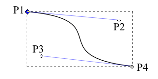
Таким образом, мы можем определить кривую Безье, которая имеет две промежуточные точки вдоль касательной, заданной углом к ​​каждой из точек. По сути, нет никаких намеков на то, где по этой касательной должны лежать две промежуточные точки, поэтому мы могли бы выбрать произвольное расстояние от двух конечных точек. Это то, что называется r в коде ниже. Выбор хорошего значения для этого параметра r является ключом к получению гладкой кривой.

import numpy as np
from scipy.special import binom
import matplotlib.pyplot as plt

bernstein = lambda n, k, t: binom(n,k)* t**k * (1.-t)**(n-k)

def bezier(points, num=200):
    N = len(points)
    t = np.linspace(0, 1, num=num)
    curve = np.zeros((num, 2))
    for i in range(N):
        curve += np.outer(bernstein(N - 1, i, t), points[i])
    return curve

class Segment():
    def __init__(self, p1, p2, angle1, angle2, **kw):
        self.p1 = p1; self.p2 = p2
        self.angle1 = angle1; self.angle2 = angle2
        self.numpoints = kw.get("numpoints", 100)
        method = kw.get("method", "const")
        if method=="const":
            self.r = kw.get("r", 1.)
        else:
            r = kw.get("r", 0.3)
            d = np.sqrt(np.sum((self.p2-self.p1)**2))
            self.r = r*d
        self.p = np.zeros((4,2))
        self.p[0,:] = self.p1[:]
        self.p[3,:] = self.p2[:]
        self.calc_intermediate_points(self.r)

    def calc_intermediate_points(self,r):
        self.p[1,:] = self.p1 + np.array([self.r*np.cos(self.angle1),
                                    self.r*np.sin(self.angle1)])
        self.p[2,:] = self.p2 + np.array([self.r*np.cos(self.angle2+np.pi),
                                    self.r*np.sin(self.angle2+np.pi)])
        self.curve = bezier(self.p,self.numpoints)


def get_curve(points, **kw):
    segments = []
    for i in range(len(points)-1):
        seg = Segment(points[i,:2], points[i+1,:2], points[i,2],points[i+1,2],**kw)
        segments.append(seg)
    curve = np.concatenate([s.curve for s in segments])
    return segments, curve


def plot_point(ax, xy, angle, r=0.3):
    ax.plot([xy[0]],[xy[1]], marker="o", ms=9, alpha=0.5, color="indigo")
    p = xy + np.array([r*np.cos(angle),r*np.sin(angle)])
    ax.plot([xy[0],p[0]], [xy[1],p[1]], color="limegreen")


if __name__ == "__main__":        
    #                   x    y    angle        
    points =np.array([[ 6.0, 0.5, 1.5],
                      [ 5.4, 1.2, 2.2],
                      [ 5.0, 1.7, 2.6],
                      [ 2.8, 2.4, 2.1],
                      [ 1.3, 3.2, 1.6],
                      [ 1.9, 3.9,-0.2],
                      [ 4.0, 3.0, 0.2],
                      [ 5.1, 3.7, 1.4]])

    fig, ax = plt.subplots()

    for point in points:
        plot_point(ax, point[:2],point[2], r=0.1)

    s1, c1 = get_curve(points, method="const", r=0.7)
    ax.plot(c1[:,0], c1[:,1], color="crimson", zorder=0, label="const 0.7 units")

    s2, c2 = get_curve(points, method="prop", r=0.3)
    ax.plot(c2[:,0], c2[:,1], color="gold", zorder=0, label="prop 30% of distance")
    plt.legend()
    plt.show()

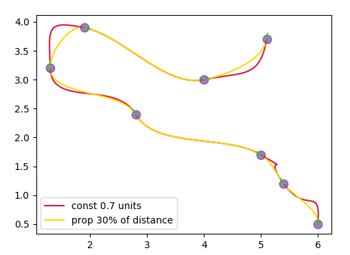
В приведенном выше сюжете сравниваются два случая. Один где r постоянно 0.7 единицы, другой где r Относительно 30% расстояния между двумя точками.