Может ли этот интеграл быть сделан численно в Matlab или Mathematica?

Question

Я хочу быть в состоянии сделать интеграл ниже численно.

где , а также , а также константы, которые для простоты могут быть установлены в 1,

Интеграл по x можно сделать аналитически вручную или с помощью Mathematica, а затем y можно сделать численно с помощью NIntegrate, но эти два метода дают разные ответы.

Аналитически:

In[160]:= ex := 2 (1 - Cos[x])

In[149]:= ey := 2 (1 - Cos[y])

In[161]:= kx := 1/(1 + Exp[ex])

In[151]:= ky := 1/(1 + Exp[ey])

In[162]:= Fn1 := 1/(2 \[Pi]) ((Cos[(x + y)/2])^2)/(ex - ey)

In[163]:= Integrate[Fn1, {x, -Pi, Pi}]

Out[163]= -(1/(4 \[Pi]))
 If[Re[y] >= \[Pi] || \[Pi] + Re[y] <= 0 || 
   y \[NotElement] Reals, \[Pi] Cos[y] - Log[-Cos[y/2]] Sin[y] + 
   Log[Cos[y/2]] Sin[y], 
  Integrate[Cos[(x + y)/2]^2/(Cos[x] - Cos[y]), {x, -\[Pi], \[Pi]}, 
   Assumptions -> ! (Re[y] >= \[Pi] || \[Pi] + Re[y] <= 0 || 
       y \[NotElement] Reals)]]

In[164]:= Fn2 := -1/(
  4 \[Pi]) ((\[Pi] Cos[y] - Log[-Cos[y/2]] Sin[y] + 
     Log[Cos[y/2]] Sin[y]) (1 - ky) ky )/(2 \[Pi])

In[165]:= NIntegrate[Fn2, {y, -Pi, Pi}]

Out[165]= -0.0160323 - 2.23302*10^-15 I

Численный метод 1:

In[107]:= Fn4 := 
 1/(4 \[Pi]^2) ((Cos[(x + y)/2])^2) (1 - ky) ky/(ex - ey)

In[109]:= NIntegrate[Fn4, {x, -Pi, Pi}, {y, -Pi, Pi}]

During evaluation of In[109]:= NIntegrate::slwcon: Numerical integration converging too slowly; suspect one of the following: singularity, value of the integration is 0, highly oscillatory integrand, or WorkingPrecision too small. >>

During evaluation of In[109]:= NIntegrate::ncvb: NIntegrate failed to converge to prescribed accuracy after 18 recursive bisections in x near {x,y} = {0.0000202323,2.16219}. NIntegrate obtained 132827.66472461013` and 19442.543606302774` for the integral and error estimates. >>

Out[109]= 132828.

Числовой 2:

In[113]:= delta = .001;
pw[x_, y_] := Piecewise[{{1, Abs[Abs[x] - Abs[y]] > delta}}, 0]

In[116]:= Fn5 := (Fn4)*pw[Cos[x], Cos[y]]

In[131]:= NIntegrate[Fn5, {x, -Pi, Pi}, {y, -Pi, Pi}]

During evaluation of In[131]:= NIntegrate::slwcon: Numerical integration converging too slowly; suspect one of the following: singularity, value of the integration is 0, highly oscillatory integrand, or WorkingPrecision too small. >>

During evaluation of In[131]:= NIntegrate::eincr: The global error of the strategy GlobalAdaptive has increased more than 2000 times. The global error is expected to decrease monotonically after a number of integrand evaluations. Suspect one of the following: the working precision is insufficient for the specified precision goal; the integrand is highly oscillatory or it is not a (piecewise) smooth function; or the true value of the integral is 0. Increasing the value of the GlobalAdaptive option MaxErrorIncreases might lead to a convergent numerical integration. NIntegrate obtained 0.013006903336304906` and 0.0006852739534086272` for the integral and error estimates. >>

Out[131]= 0.0130069

Так что ни один из численных методов не дает -0.0160323, Я понимаю, почему - первый метод имеет проблемы с бесконечностями, вызванными знаменателем, а второй метод эффективно удаляет ту часть интеграла, которая вызывает проблемы. Но я хотел бы иметь возможность интегрировать другой интеграл (более сложный x, y а также z) который нельзя упростить аналитически. Приведенный выше интеграл дает мне возможность проверить любой новый метод, так как я знаю, каким должен быть ответ.

Answer 1

Если я не записал интегральную ошибку, это должно сделать работу:

n[x_] := 1/(1 + Exp[eps[x]])
eps[x_] := 2(1 - Cos[x])
.25/(2*Pi)^2*NIntegrate[
    Cos[(x + y)/
     2]^2 ((1 - n[y]) n[y] - (1 - n[x]) n[x])/(Cos[y] - Cos[x]),
    {x, -Pi, Pi},
    {y, -Pi, Pi},
    Exclusions -> {Cos[x] == Cos[y]}
  ]

дающий 0.0130098,

Хорошо, я думаю, что самый быстрый способ объяснить это так:

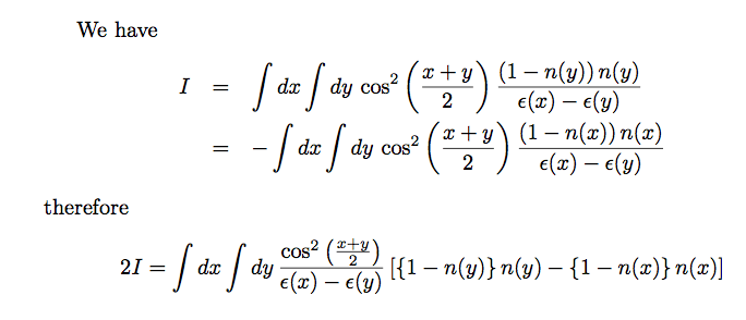
переходя от первой ко второй строке первого уравнения, я только что переименовал у в х (область интеграции симметрична, так что все в порядке). Затем я добавил два (эквивалентных) выражения для I, чтобы получить 2I, и что я численно интегрирую, так это. Дело в том, что числитель и знаменатель исчезают в одних и тех же точках, поэтому на самом деле Exclusions опция не нужна. Обратите внимание, что в моем наброске метода выше я опустил 1/(4*Pi^2) для краткости (или из-за лени, в зависимости от точки зрения).