Начальная визуализация наборов данных в команде Scikit - head()
Рассматривая потенциальную эквивалентность Python для R для обработки данных, я работаю над основами. В частности, при загрузке базы данных, такой как Iris в R, простая команда head() производит красивую распечатку на экране:
head(iris)
  Sepal.Length Sepal.Width Petal.Length Petal.Width Species
1          5.1         3.5          1.4         0.2  setosa
2          4.9         3.0          1.4         0.2  setosa
3          4.7         3.2          1.3         0.2  setosa
4          4.6         3.1          1.5         0.2  setosa
5          5.0         3.6          1.4         0.2  setosa
6          5.4         3.9          1.7         0.4  setosa
Scikit включает этот набор данных, но если бы я не был знаком с ним и пытался просто взглянуть на то, как он выглядит, это были бы первые неудачные результаты:
from sklearn.datasets import load_iris
iris = load_iris()
iris
{'DESCR': 'Iris Plants Database\n\nNotes\n-----\nData Set Characteristics:\n    :Number of Instances: 150 (50 in each of three classes)\n    :Number of Attributes: 4 numeric, predictive attributes and the class\n    :Attribute Information:\n        - sepal length in cm\n        - sepal width in cm\n        - petal length in cm\n        - petal width in cm\n        - class:\n                - Iris-Setosa\n                - Iris-Versicolour\n                - Iris-Virginica\n    :Summary Statistics:\n\n    ============== ==== ==== ======= ===== ====================\n                    Min  Max   Mean    SD   Class Correlation\n    ============== ==== ==== ======= ===== ====================\n    sepal length:   4.3  7.9   5.84   0.83    0.7826\n    sepal width:    2.0  4.4   3.05   0.43   -0.4194\n    petal length:   1.0  6.9   3.76   1.76    0.9490  (high!)\n    petal width:    0.1  2.5   1.20  0.76     0.9565  (high!)\n    ============== ==== ==== ======= ===== ====================\n\n    :Missing Attribute Values: None\n    :Class Distribution: 33.3% for each of 3 classes.\n    :Creator: R.A. Fisher\n    :Donor: Michael Marshall (MARSHALL%PLU@io.arc.nasa.gov)\n    :Date: July, 1988\n\nThis is a copy of UCI ML iris datasets.\nhttp://archive.ics.uci.edu/ml/datasets/Iris\n\nThe famous Iris database, first used by Sir R.A Fisher\n\nThis is perhaps the best known database to be found in the\npattern recognition literature.  Fisher\'s paper is a classic in the field and\nis referenced frequently to this day.  (See Duda & Hart, for example.)  The\ndata set contains 3 classes of 50 instances each, where each class refers to a\ntype of iris plant.  One class is linearly separable from the other 2; the\nlatter are NOT linearly separable from each other.\n\nReferences\n----------\n   - Fisher,R.A. "The use of multiple measurements in taxonomic problems"\n     Annual Eugenics, 7, Part II, 179-188 (1936); also in "Contributions to\n     Mathematical Statistics" (John Wiley, NY, 1950).\n   - Duda,R.O., & Hart,P.E. (1973) Pattern Classification and Scene Analysis.\n     (Q327.D83) John Wiley & Sons.  ISBN 0-471-22361-1.  See page 218.\n   - Dasarathy, B.V. (1980) "Nosing Around the Neighborhood: A New System\n     Structure and Classification Rule for Recognition in Partially Exposed\n     Environments".  IEEE Transactions on Pattern Analysis and Machine\n     Intelligence, Vol. PAMI-2, No. 1, 67-71.\n   - Gates, G.W. (1972) "The Reduced Nearest Neighbor Rule".  IEEE Transactions\n     on Information Theory, May 1972, 431-433.\n   - See also: 1988 MLC Proceedings, 54-64.  Cheeseman et al"s AUTOCLASS II\n     conceptual clustering system finds 3 classes in the data.\n   - Many, many more ...\n',
 'data': array([[ 5.1,  3.5,  1.4,  0.2],
        [ 4.9,  3. ,  1.4,  0.2],
        [ 4.7,  3.2,  1.3,  0.2],
        [ 4.6,  3.1,  1.5,  0.2],
        [ 5. ,  3.6,  1.4,  0.2],
        [ 5.4,  3.9,  1.7,  0.4],
        [ 4.6,  3.4,  1.4,  0.3],
        [ 5. ,  3.4,  1.5,  0.2],
        [ 4.4,  2.9,  1.4,  0.2],
        [ 4.9,  3.1,  1.5,  0.1],
        [ 5.4,  3.7,  1.5,  0.2],
        [ 4.8,  3.4,  1.6,  0.2],
        [ 4.8,  3. ,  1.4,  0.1],
        [ 4.3,  3. ,  1.1,  0.1],
        [ 5.8,  4. ,  1.2,  0.2],
        [ 5.7,  4.4,  1.5,  0.4],
        [ 5.4,  3.9,  1.3,  0.4],
        [ 5.1,  3.5,  1.4,  0.3],
        [ 5.7,  3.8,  1.7,  0.3],
        [ 5.1,  3.8,  1.5,  0.3],
        [ 5.4,  3.4,  1.7,  0.2],
        [ 5.1,  3.7,  1.5,  0.4],
        [ 4.6,  3.6,  1. ,  0.2],
        [ 5.1,  3.3,  1.7,  0.5],
        [ 4.8,  3.4,  1.9,  0.2],
        [ 5. ,  3. ,  1.6,  0.2],
        [ 5. ,  3.4,  1.6,  0.4],
        [ 5.2,  3.5,  1.5,  0.2],
        [ 5.2,  3.4,  1.4,  0.2],
        [ 4.7,  3.2,  1.6,  0.2],
        [ 4.8,  3.1,  1.6,  0.2],
        [ 5.4,  3.4,  1.5,  0.4],
        [ 5.2,  4.1,  1.5,  0.1],
        [ 5.5,  4.2,  1.4,  0.2],
        [ 4.9,  3.1,  1.5,  0.1],
        [ 5. ,  3.2,  1.2,  0.2],
        [ 5.5,  3.5,  1.3,  0.2],
        [ 4.9,  3.1,  1.5,  0.1],
        [ 4.4,  3. ,  1.3,  0.2],
        [ 5.1,  3.4,  1.5,  0.2],
        [ 5. ,  3.5,  1.3,  0.3],
        [ 4.5,  2.3,  1.3,  0.3],
        [ 4.4,  3.2,  1.3,  0.2],
        [ 5. ,  3.5,  1.6,  0.6],
        [ 5.1,  3.8,  1.9,  0.4],
        [ 4.8,  3. ,  1.4,  0.3],
        [ 5.1,  3.8,  1.6,  0.2],
        [ 4.6,  3.2,  1.4,  0.2],
        [ 5.3,  3.7,  1.5,  0.2],
        [ 5. ,  3.3,  1.4,  0.2],
        [ 7. ,  3.2,  4.7,  1.4],
        [ 6.4,  3.2,  4.5,  1.5],
        [ 6.9,  3.1,  4.9,  1.5],
        [ 5.5,  2.3,  4. ,  1.3],
        [ 6.5,  2.8,  4.6,  1.5],
        [ 5.7,  2.8,  4.5,  1.3],
        [ 6.3,  3.3,  4.7,  1.6],
        [ 4.9,  2.4,  3.3,  1. ],
        [ 6.6,  2.9,  4.6,  1.3],
        [ 5.2,  2.7,  3.9,  1.4],
        [ 5. ,  2. ,  3.5,  1. ],
        [ 5.9,  3. ,  4.2,  1.5],
        [ 6. ,  2.2,  4. ,  1. ],
        [ 6.1,  2.9,  4.7,  1.4],
        [ 5.6,  2.9,  3.6,  1.3],
        [ 6.7,  3.1,  4.4,  1.4],
        [ 5.6,  3. ,  4.5,  1.5],
        [ 5.8,  2.7,  4.1,  1. ],
        [ 6.2,  2.2,  4.5,  1.5],
        [ 5.6,  2.5,  3.9,  1.1],
        [ 5.9,  3.2,  4.8,  1.8],
        [ 6.1,  2.8,  4. ,  1.3],
        [ 6.3,  2.5,  4.9,  1.5],
        [ 6.1,  2.8,  4.7,  1.2],
        [ 6.4,  2.9,  4.3,  1.3],
        [ 6.6,  3. ,  4.4,  1.4],
        [ 6.8,  2.8,  4.8,  1.4],
        [ 6.7,  3. ,  5. ,  1.7],
        [ 6. ,  2.9,  4.5,  1.5],
        [ 5.7,  2.6,  3.5,  1. ],
        [ 5.5,  2.4,  3.8,  1.1],
        [ 5.5,  2.4,  3.7,  1. ],
        [ 5.8,  2.7,  3.9,  1.2],
        [ 6. ,  2.7,  5.1,  1.6],
        [ 5.4,  3. ,  4.5,  1.5],
        [ 6. ,  3.4,  4.5,  1.6],
        [ 6.7,  3.1,  4.7,  1.5],
        [ 6.3,  2.3,  4.4,  1.3],
        [ 5.6,  3. ,  4.1,  1.3],
        [ 5.5,  2.5,  4. ,  1.3],
        [ 5.5,  2.6,  4.4,  1.2],
        [ 6.1,  3. ,  4.6,  1.4],
        [ 5.8,  2.6,  4. ,  1.2],
        [ 5. ,  2.3,  3.3,  1. ],
        [ 5.6,  2.7,  4.2,  1.3],
        [ 5.7,  3. ,  4.2,  1.2],
        [ 5.7,  2.9,  4.2,  1.3],
        [ 6.2,  2.9,  4.3,  1.3],
        [ 5.1,  2.5,  3. ,  1.1],
        [ 5.7,  2.8,  4.1,  1.3],
        [ 6.3,  3.3,  6. ,  2.5],
        [ 5.8,  2.7,  5.1,  1.9],
        [ 7.1,  3. ,  5.9,  2.1],
        [ 6.3,  2.9,  5.6,  1.8],
        [ 6.5,  3. ,  5.8,  2.2],
        [ 7.6,  3. ,  6.6,  2.1],
        [ 4.9,  2.5,  4.5,  1.7],
        [ 7.3,  2.9,  6.3,  1.8],
        [ 6.7,  2.5,  5.8,  1.8],
        [ 7.2,  3.6,  6.1,  2.5],
        [ 6.5,  3.2,  5.1,  2. ],
        [ 6.4,  2.7,  5.3,  1.9],
        [ 6.8,  3. ,  5.5,  2.1],
        [ 5.7,  2.5,  5. ,  2. ],
        [ 5.8,  2.8,  5.1,  2.4],
        [ 6.4,  3.2,  5.3,  2.3],
        [ 6.5,  3. ,  5.5,  1.8],
        [ 7.7,  3.8,  6.7,  2.2],
        [ 7.7,  2.6,  6.9,  2.3],
        [ 6. ,  2.2,  5. ,  1.5],
        [ 6.9,  3.2,  5.7,  2.3],
        [ 5.6,  2.8,  4.9,  2. ],
        [ 7.7,  2.8,  6.7,  2. ],
        [ 6.3,  2.7,  4.9,  1.8],
        [ 6.7,  3.3,  5.7,  2.1],
        [ 7.2,  3.2,  6. ,  1.8],
        [ 6.2,  2.8,  4.8,  1.8],
        [ 6.1,  3. ,  4.9,  1.8],
        [ 6.4,  2.8,  5.6,  2.1],
        [ 7.2,  3. ,  5.8,  1.6],
        [ 7.4,  2.8,  6.1,  1.9],
        [ 7.9,  3.8,  6.4,  2. ],
        [ 6.4,  2.8,  5.6,  2.2],
        [ 6.3,  2.8,  5.1,  1.5],
        [ 6.1,  2.6,  5.6,  1.4],
        [ 7.7,  3. ,  6.1,  2.3],
        [ 6.3,  3.4,  5.6,  2.4],
        [ 6.4,  3.1,  5.5,  1.8],
        [ 6. ,  3. ,  4.8,  1.8],
        [ 6.9,  3.1,  5.4,  2.1],
        [ 6.7,  3.1,  5.6,  2.4],
        [ 6.9,  3.1,  5.1,  2.3],
        [ 5.8,  2.7,  5.1,  1.9],
        [ 6.8,  3.2,  5.9,  2.3],
        [ 6.7,  3.3,  5.7,  2.5],
        [ 6.7,  3. ,  5.2,  2.3],
        [ 6.3,  2.5,  5. ,  1.9],
        [ 6.5,  3. ,  5.2,  2. ],
        [ 6.2,  3.4,  5.4,  2.3],
        [ 5.9,  3. ,  5.1,  1.8]]),
 'feature_names': ['sepal length (cm)',
  'sepal width (cm)',
  'petal length (cm)',
  'petal width (cm)'],
 'target': array([0, 0, 0, 0, 0, 0, 0, 0, 0, 0, 0, 0, 0, 0, 0, 0, 0, 0, 0, 0, 0, 0, 0,
        0, 0, 0, 0, 0, 0, 0, 0, 0, 0, 0, 0, 0, 0, 0, 0, 0, 0, 0, 0, 0, 0, 0,
        0, 0, 0, 0, 1, 1, 1, 1, 1, 1, 1, 1, 1, 1, 1, 1, 1, 1, 1, 1, 1, 1, 1,
        1, 1, 1, 1, 1, 1, 1, 1, 1, 1, 1, 1, 1, 1, 1, 1, 1, 1, 1, 1, 1, 1, 1,
        1, 1, 1, 1, 1, 1, 1, 1, 2, 2, 2, 2, 2, 2, 2, 2, 2, 2, 2, 2, 2, 2, 2,
        2, 2, 2, 2, 2, 2, 2, 2, 2, 2, 2, 2, 2, 2, 2, 2, 2, 2, 2, 2, 2, 2, 2,
        2, 2, 2, 2, 2, 2, 2, 2, 2, 2, 2, 2]),
 'target_names': array(['setosa', 'versicolor', 'virginica'],
       dtype='<U10')}
Tough! Я мог бы попытаться преобразовать набор данных в фрейм данных, используя панд...
from pandas import *
iris = load_iris()
df = DataFrame(iris.data, columns=iris.feature_names)
df.head()
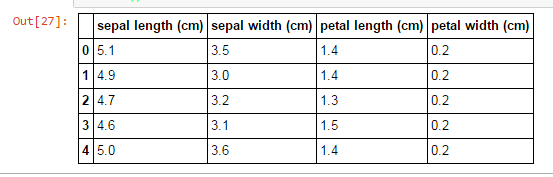
который, если не считать эстетики (уродливая рамка и жирный шрифт - субъективный), больше похож на вывод R, за исключением отсутствия Species колонка.
Что я делаю неправильно?
2 ответа
Для аналогичного вывода R-головы () может быть сделано с помощью Seaborne в Scikit-learn. Это в основном то, как оно хранится в Scikit-learn и Seaborne.
import seaborn as sns

iris = sns.load_dataset("iris")

print(iris.head())

   sepal_length  sepal_width  petal_length  petal_width species
0           5.1          3.5           1.4          0.2  setosa
1           4.9          3.0           1.4          0.2  setosa
2           4.7          3.2           1.3          0.2  setosa
3           4.6          3.1           1.5          0.2  setosa
4           5.0          3.6           1.4          0.2  setosa
При использовании Jupyter Notebook по умолчанию датафрейм будет представлен в виде таблицы html. использование print чтобы получить текст.
df = pd.DataFrame(
    iris['data'], columns=iris['feature_names']
).assign(Species=iris['target_names'][iris['target']])

with pd.option_context('expand_frame_repr', False):
    print(df.head())

   sepal length (cm)  sepal width (cm)  petal length (cm)  petal width (cm) Species
0                5.1               3.5                1.4               0.2  setosa
1                4.9               3.0                1.4               0.2  setosa
2                4.7               3.2                1.3               0.2  setosa
3                4.6               3.1                1.5               0.2  setosa
4                5.0               3.6                1.4               0.2  setosa